8.2.   Recently Added Features

This page contains significant features recently added to the data cleaning pipeline - most recent at the top. Details can also be found in the full documentation (updated on this website soon).

Watch this space for third stage changes coming soon…

Updated: 10 February 2025

New Overwrite feature:

Sometimes we need to overwrite multiple properties for one or more traces that have already been created e.g. in an include file. The global variables feature allows this, however, once this section becomes long with many trace property tweaks, it can become very hard to troubleshoot, and in these cases having all the information for one trace together is more desirable.

Instead of using global variables you can duplicate the full trace ([Trace] ... [End]), and in your site-specific first stage INI file, put this duplicate after the line of code where the include file is called that contains your original trace. Note the additional Overwrite property highlighted in yellow:

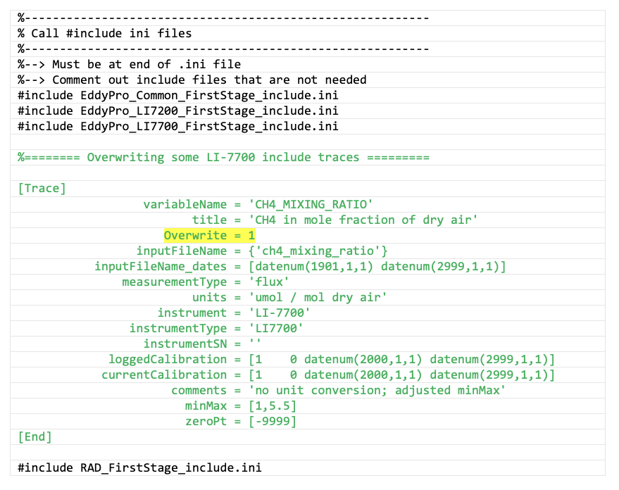
Location within site-specific INI file to put duplicate trace for overwriting a trace previously defined in an include INI file. In this case, we want to overwrite the CH4_MIXING_RATIO trace that was originally defined in EddyPro_LI7700_FirstStage_include.ini. Yellow highlighting shows the syntax for the “overwrite” property.

There are three overwrite options:

• 0 = do not overwrite with this trace. This is the default setting. If you do not include the Overwrite parameter, the pipeline assumes this option. If you have a duplicate trace you will get an error during cleaning (Example 1):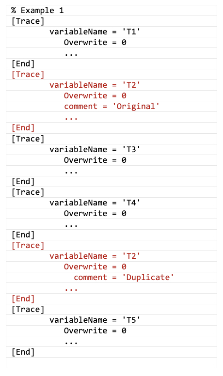

  

• 1 = overwrite traces having the same variableName and also with Overwrite = 0 setting. This puts the duplicate data where the original data was, i.e., complete overwrite, first trace gone. Use this setting if you want your duplicate T2 available to use in a later variable such as T3, T4, T5, etc. (Example 2):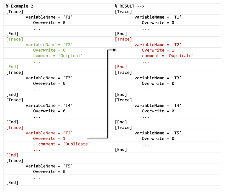

  

• 2 = overwrite traces having the same variableName and with Overwrite = 0 setting. This takes advantage of the “position” of the duplicate trace. Use this setting if you want a later variable such as T3 or T4 available to use in T2.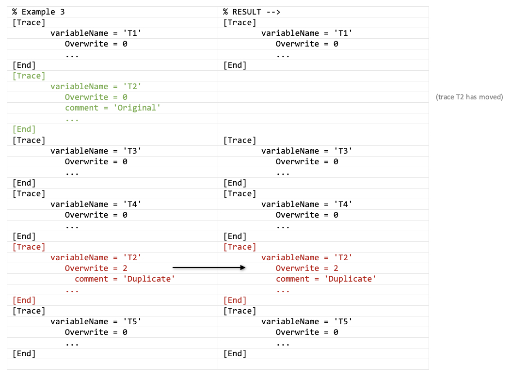

  

New postEvaluate property:

More complex user-defined processing can be applied in the first stage to any trace using the very useful “Evaluate” and new “postEvaluate” options. Matlab functions (user-written or from Biomet.net) can be called from this statement. Multiple Matlab statements can be called from within the “Evaluate” or “postEvaluate” strings. They can be used to derive variables from available data, flag variables to remove bad data, or to calculate new useful variables. Here is an Evaluate example for removing outliers from a trace:

Evaluate = 'wlen=24;thres=4;TA_1_1_1 = run_std_dev(TA_1_1_1,clean_tv,wlen,thres);'

The Evaluate property is executed for all traces before any other cleaning properties, e.g., minMax, calibration, etc.. In contrast, the newer postEvaluate property is executed in the first stage after all other cleaning is done.

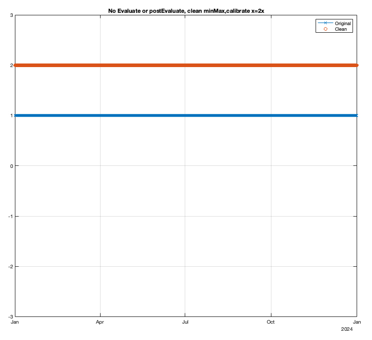
Generally speaking, the order of operations is: Evaluate –> other cleaning (e.g., minMax, calibration) –> postEvaluate. This is regardless of the order that they appear within [Trace] ... [End]. The following series of examples show how the Evaluate and postEvaluate statements work in relation to the other cleaning properties. For each example the input (Original) is an array of ones, and both the “Original” and first-stage “Clean” data are plotted in the result.

Example 1: Only minMax and calibration, no Evaluate or postEvaluate statements

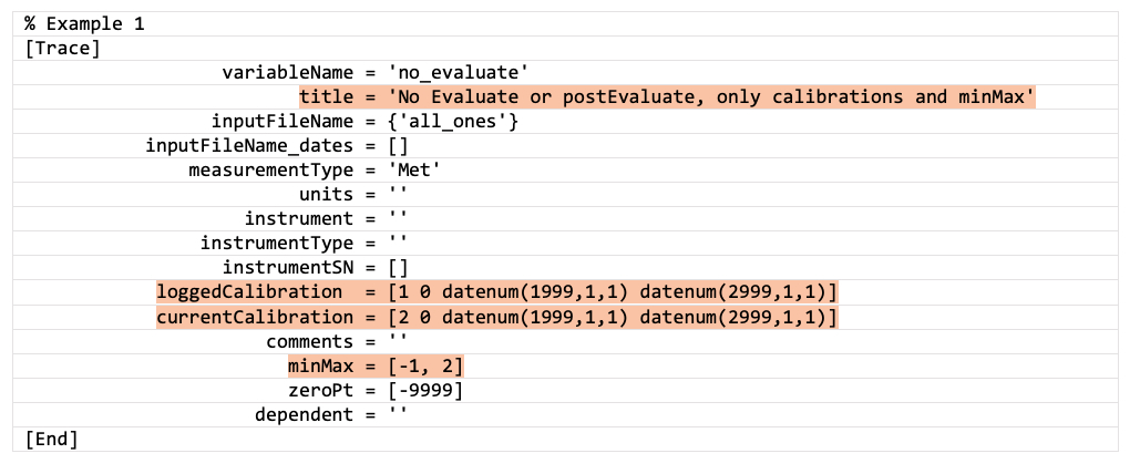
Result: x = 2x [calibrated]

Example 2: Evaluate, minMax and calibration, no postEvaluate statement

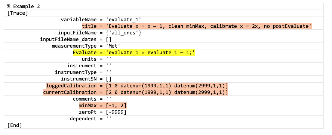
Result: x = (x - 1)*2 [Evaluate first, then calibrate]

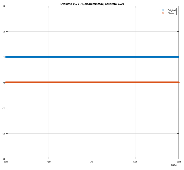
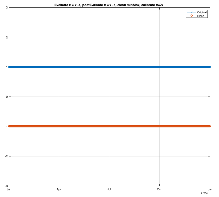
Example 3: minMax and calibration, postEvaluate statement, no Evaluate statement

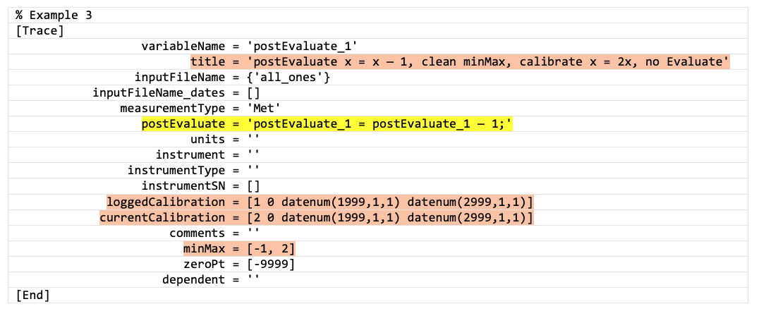
Result: x = 2x - 1 [calibrate, then postEvaluate]

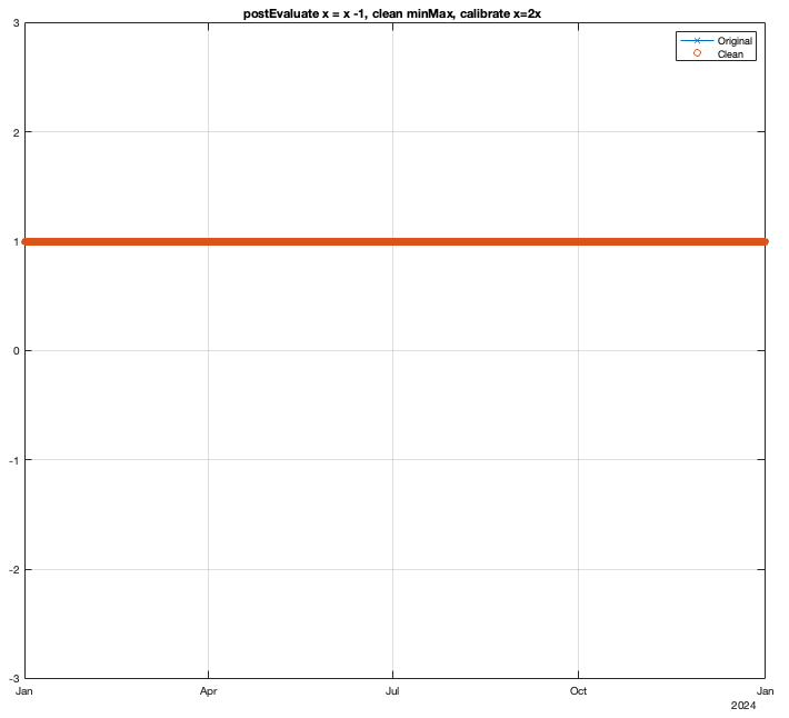
Example 4: minMax and calibration, both Evaluate and postEvaluate statements

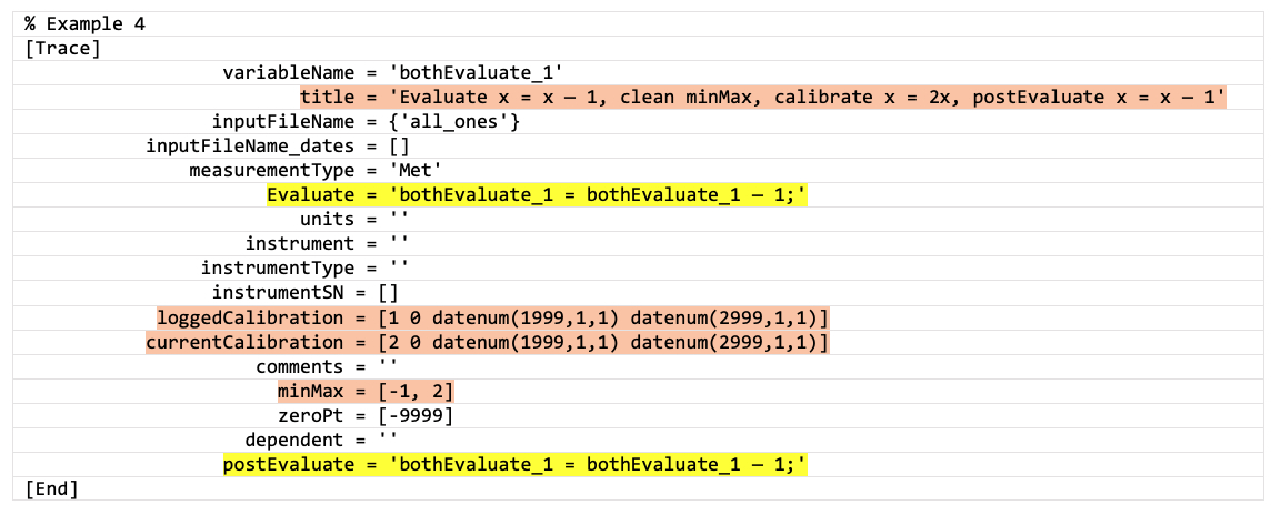
Result: x = (x - 1)*2 - 1 [Evaluate, then calibrate, then postEvaluate]