5.1.   Quick Start: Create Database from Raw Data and Visualize Contents

This section provides a generic, quick-start example that converts (1) EddyPro raw data output, and (2) Campbell Scientific TOA5 output, to a formatted database ready to be processed using the standardised libraries (i.e., Biomet.net). We also present some examples of how to quickly check the contents of your new database.

Create database using data from your own site(s)

As previously mentioned, we will follow an example that focuses on flux-related EddyPro and met-related Campbell Scientific output data:

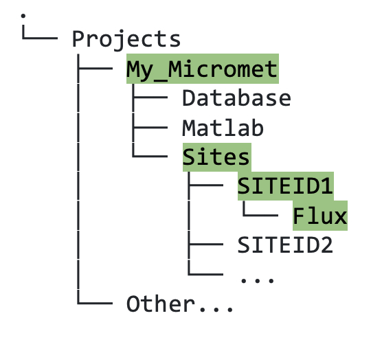
1. First, in your newly created Sites directory, within the relevant SITEID directory, create a new Flux folder (figure 5.1).

   

   Figure 5.1. Directory tree showing file path to the location where raw flux data for site with SITEID1 should be stored.

2. Copy your EddyPro raw output data to this Flux folder. This data will remain untouched so that you always have a local copy of the original data.

3. Now, create a Met folder within the same SITEID directory (SITEID1 in this example), and copy your Campbell Scientific TOA5 data for this site to this Met folder.

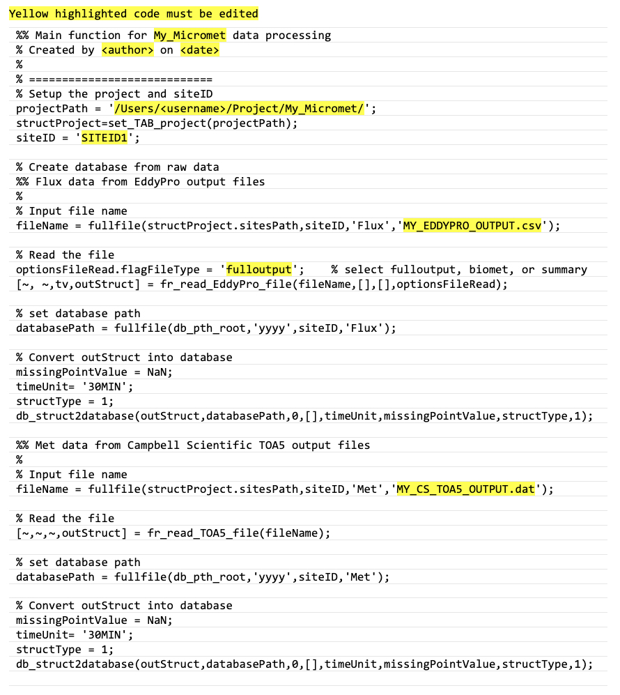
4. In your <projectPath>/Matlab folder, create one new “main” Matlab file that will act as a “do-it-all” script. You can name this file however you like; we advise making it meaningful and including the word “Main”. The example given here (figure 5.2) is named DataCleaning_Main.m (you can make your filename less generic) — it will first create the database, and later you can add the code for data cleaning. This script can be copied section by section from the code block at the bottom of this page.

   

   Figure 5.2. Matlab code to create database from raw EddyPro output and Campbell Scientific logger meteorological data. Yellow highlighted text should be edited.

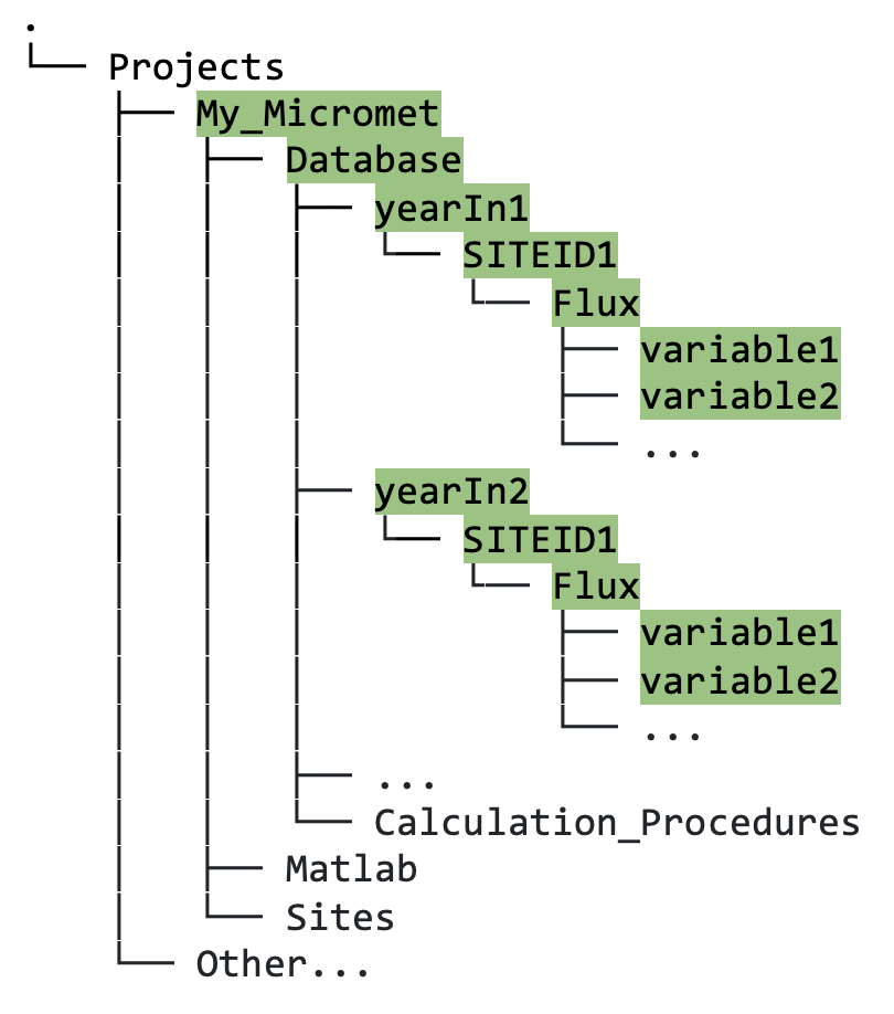
5. Next, run your “Main” Matlab program; you should see some data output in your Database directory. Data is grouped by year, then by site, then by data type, e.g., Flux or Met (figure 5.3; Met data not shown here).

   

   Figure 5.3. Directory tree showing file path to output in Database directory following database conversion.

Your data is now in a format ready for cleaning using the pipeline.

Visualize contents of new database

Here are some quick tips to inspect the data in your newly created database, all within Matlab:

1. plotApp function:
   Simply type plotApp on the Matlab command line, and it will open an app that can compare traces from the same and different cleaning stages (once you have completed those), databases, and also produce statistical plots and outputs. More details of this and other visualization tools are described at length in section 7.

2. gui_Browse_folder function:

    pth = biomet_path(yearIn, 'SITEID1', 'Flux')  % define path to folder you wish to browse
    gui_Browse_Folder(pth)
    

   This function opens a Matlab app that looks in the Flux folder for SITEID1 for a specific year (as defined in the biomet_path function input parameters) and plots each variable in turn. You can scroll through or use the dropdown in order to check that your data looks reasonable and as expected.

3. Load one trace, e.g., co2_mixing_ratio and plot it.

    %% Load one trace and plot it
    pth = biomet_path(yearIn,'SITEID1','Flux');   
    tv = read_bor(fullfile(pth,'clean_tv'),8);      % load the time vector (Matlab's datenum format)
    tv_dt = datetime(tv,'convertfrom','datenum');   % convert to Matlab's datetime object
    x = read_bor(fullfile(pth,'co2_mixing_ratio')); % load co2_mixing_ratio from SITEID1/Flux folder
    plot(tv_dt,x)                                   % plot data
    grid on;zoom on
    

---

DataCleaning_Main.m template script for copying one section at a time (see Figure 5.2 for necessary edits, highlighted yellow):

%% Main function for My_Micromet data processing
% Created by <author> on <date>
% 
% ============================
% Setup the project and siteID
projectPath = '/Users/<username>/Project/My_Micromet';
structProject=set_TAB_project(projectPath);
siteID = 'SITEID1';

% Create database from raw data
%% Flux data from EddyPro output files
%
% Input file name
fileName = fullfile(structProject.sitesPath,siteID,'Flux','MY_EDDYPRO_OUTPUT.csv');

% Read the file 
optionsFileRead.flagFileType = 'fulloutput';    % select fulloutput, biomet, or summary
[~, ~,tv,outStruct] = fr_read_EddyPro_file(fileName,[],[],optionsFileRead);

% set database path 
databasePath = fullfile(db_pth_root,'yyyy',siteID,'Flux'); 

% Convert outStruct into database 
missingPointValue = NaN; 
timeUnit= '30MIN'; 
structType = 1; 
db_struct2database(outStruct,databasePath,0,[],timeUnit,missingPointValue,structType,1); 

%% Met data from Campbell Scientific TOA5 output files
%
% Input file name
fileName = fullfile(structProject.sitesPath,siteID,'Met','MY_CS_TOA5_OUTPUT.dat');

% Read the file 
[~,~,~,outStruct] = fr_read_TOA5_file(fileName); 

% set database path 
databasePath = fullfile(db_pth_root,'yyyy',siteID,'Met'); 

% Convert outStruct into database 
missingPointValue = NaN; 
timeUnit= '30MIN'; 
structType = 1; 
db_struct2database(outStruct,databasePath,0,[],timeUnit,missingPointValue,structType,1);