3. Data Cleaning Principles
This section outlines the data cleaning principles and processes that should be followed closely and applied at each of the three stages, as well as other relevant information.

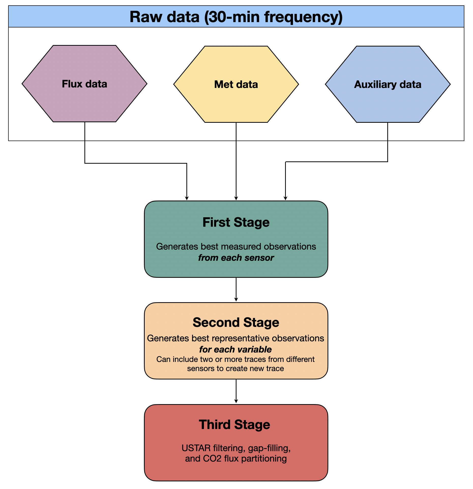
Figure 3. Chart outlining the data cleaning principles followed in the pipeline.
First Stage
Principle: During the first stage of data cleaning, we want to keep the best measured data values from each sensor, i.e., a user looking for the best measurements from a particular sensor would want to use the first stage data. Missing data points for periods of more than one half-hour will not be gap-filled in any way.
At the most basic level, the first stage collects the raw data, applies min/max filtering, assigns consistent variable names in line with Ameriflux guidelines as far as possible, and moves the relevant files to a
Cleanfolder in preparation for stage two. This folder will be created automatically if it does not already exist.The data are stored as binary files in “single-precision floating-point format” (aka float 32), which importantly means they are readable in most common computer languages and software.
Second Stage
Principle: The second stage focuses on creating the best measured data values for each particular property/variable. For example, if there are two (or more) collocated temperature sensors at the same height e.g., 2 metres above ground level, the second stage is intended to create the “best” trace using both (all) sensors, with the highest precision/accuracy and the fewest missing points. By default, it does this by averaging the traces, and gap-filling by using linear regression. Optionally, data can be gap-filled using a nearby climate station, or one of your own nearby stations if you have one. (Other gap-filling methods, such as using reanalysis data, are currently under development.)
In practice, the second stage collects the first stage data, generates the “best” observation for each variable and moves the relevant files to a “Clean/SecondStage” folder in preparation for the third stage.
Third Stage
- Principle: USTAR filtering, gap-filling, and CO2 flux partitioning.
- The third stage collects the second stage data and implements USTAR filtering, gap-filling, and flux partitioning procedures. For this we use the R package REddyProc. Biomet.net functions allow Matlab to interface with R, so all three stages are run directly from Matlab. For more machine learning approaches to gap-filling, we also implement the random forest approach described in the paper by Kim et al. (2020). Additional methane gap-filling processes currently not part of the pipeline are described here, with instructions here.
We achieve these principles by setting up various configuration files used in each stage. This process is described later (section 4.3), but there are a few more steps to complete before that. Next, you will set up your project directory structure and then configure it to work with the Biomet.net library.