full_doc_create_database_from_raw_data_inspect_outputs

5.2. Full Documentation: Create Database from Raw Data and Inspect Contents

This section complements the quick-start set up in section 4.2.

On this page:

Best practices
Useful information on creating your database
Create Database From Multiple Input Files and Updates for Continuous Operational Sites
Create Database Using Data from Canadian Meteorological Stations
Create Database Using Data from U.S. Meteorological Stations
Visualize and inspect your newly created database

Best practices

The best-practice approach for each project is to have one “main” script for data processing (e.g., DataCleaning_Main.m). This script should contain all the steps that are needed to go from raw data to the final cleaned and gap-filled Ameriflux data set:

Obtaining/downloading the raw data (not covered here, we assume you have your own systems for obtaining datalogger output from your sites);
Creating the database in the appropriate format (this current subsection);
Applying the data-cleaning stages (subsections 5.3, 5.4, and 5.5).

Each flux site is unique with its own sensors, data loggers, and data archiving formats (such as EddyPro output files, TOA5 Campbell Scientific files, Ameriflux CSV files, to name a few). The purpose of step 2 is to convert from such a site-specific dataset to a generic dataset ready to be processed using the standardised libraries (i.e., Biomet.net). These “generic” binary files can be read by most computer languages, by design, meaning they are suitable for the Biomet library which contains code written in Matlab, R, and Python.

If you need help getting started with your “main” computer program, a sample Matlab script is provided in the quick-start guide (section 4.2, under “Sample Code”). With that DataCleaning_Main.m script the entire data processing process is documented and it can be easily replicated. Insert as many informative comments as you can - it will help if the process needs to be reviewed later on or the project is handed over to another person. When working with your own data, especially for the first time using the pipeline, we still recommend following the steps in the tutorial as they also outline where to put your raw data files, and other important tasks.

Useful information on creating your database

Determine the data format/source of raw data in your Sites directory.
Use standard existing function(s) from the Biomet.net library, which you have already cloned/downloaded, to convert your raw data and create the database in Database directory. Examples of functions that can read your data and be used in your “main” script are as follows:
1. db_struct2database (create database from Matlab structure; flux or met data);
2. fr_read_EddyPro_file (create database from EddyPro output; flux data);
3. fr_read_TOA5_file (create database from TOA5 Campbell Scientific ASCII files);
4. fr_read_generic_data_file (create database from most file formats).

The relevant function, when run in matlab, will create subdirectories named by data year (yearIn), then by SITEID (i.e., SITEIDs are grouped by year), as follows: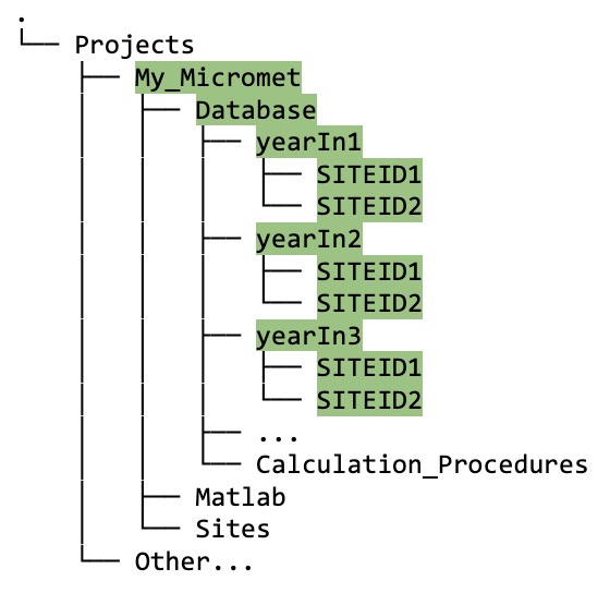

Figure 5.2A. Directory tree showing structure of Database folder for multiple years and multiple sites under one project.
The SITEID subdirectories will be populated with data (e.g., Flux and Met if these data types exist) for the appropriate year, stored as binary files ready for cleaning. The green highlighting in figure 5.2A shows an example with three years of data from two different sites.
The clean_tv file is automatically created, and will be located in each Raw/Clean folder. This a standardized time vector of 30-minute frequency. This formats the timestamp of each record in Local Standard Time (LST; as required by AmeriFlux).

We advise you to generalize your scripts as far as possible, based on the sites and data that you have, and remember to document your code thoroughly.

Creating Database from Multiple Input Files and Updates for Continuous Operational Sites

In real applications, it is likely that users will have multiple input files from Flux and Met stations (daily, monthly, or annual files). It is also very often the case with active sites that new files are continuously being downloaded from the site and added to the data folder.

To facilitate data processing in those cases we use specialized functions that can deal with multiple files and keep track of which files have changes since the last database update and update only those. That way raw data folders can contain thousands of files without affecting the speed of the database updates.

Updating Flux data

Here is an example of how to update database from any files in the Sites/siteID/Flux folder that match a file pattern (in this case eddypro_TUT_*.csv).

%% Processing multiple EddyPro files from the same folder 
projectPath = 'E:\Pipeline_Projects\TUT_Project'; 
structProject = set_TAB_project(projectPath); 
siteID = 'TUT'; 
FluxDatabase_Pth = fullfile(structProject.databasePath, 'yyyy', siteID,'Flux'); 
progressListPth = fullfile(structProject.sitesPath,siteID,'Flux','EddyPro_progressList.mat'); 
filePattern = fullfile(structProject.sitesPath,siteID,'Flux','eddypro_TUT_*.csv'); 
optionsFileRead.flagFileType = 'fulloutput'; 
missingPointValue = NaN; 
timeUnit = '30MIN'; 
[nFiles,nHHours]=fr_EddyPro_database(filePattern,progressListPth,FluxDatabase_Pth,[],timeUnit,missingPointValue,optionsFileRead); 
fprintf('  %s - Flux  Number of files processed = %d, Number of HHours = %d\n',siteID,nFiles,nHHours);

You will need to change the projectPath and maybe also the filePattern, if yours is different, before running this code.

Updating Met data

If we then wanted to process met data from Sites/siteID/Met folder (using the same projectPath, structProject and siteID) with the file-name pattern matching: TUT_MET.* we could run the following script:

%% Processing multiple TOA5 files from the same folder 
MetDatabase_Pth = fullfile(structProject.databasePath, 'yyyy', siteID,'Met'); 
progressListPth = fullfile(structProject.sitesPath,siteID,'Met','Met_progressList.mat'); 
filePattern = fullfile(structProject.sitesPath,siteID,'Met','TUT_MET.*'); 
missingPointValue = NaN; 
timeUnit = '30MIN'; 
[nFiles,nHHours]=fr_TOA5_database(filePattern,progressListPth,MetDatabase_Pth,[],timeUnit,missingPointValue);  
fprintf('  %s - Met  Number of files processed = %d, Number of HHours = %d\n',siteID,nFiles,nHHours);

If we run the same sequence twice (fr_TOA5_database or fr_EddyPro_database as shown above), the second time the number of files processed would be zero assuming that there were no new files added to the Sites folder between the two runs. If on the other hand, one of the files changed, the function would process it. That is how real-time data gets processed in this data pipeline.

Other examples of Biomet.net functions that update data continuously, and can be written into a script as previously shown, are as follows:

fr_HOBO_database (continuously create database from HOBO met data);
fr_SmartFlux_database (continuously create database from SmartFlux output; flux data);
fr_SoilFluxPro_database (continuously create database from SoilFluxPro output data).

Create Database Using Data from Canadian Meteorological Stations

Data from Canadian meteorological stations [operational climate stations run by Environment and Climate Change Canada (ECCC)] can be used for gap-filling met data for Canadian flux sites that are in close proximity. If you have gaps in your met data, you can search for nearby climate stations as follows:

To find the closest Environment ECCC stations to your flux site, first go to this website: https://climate.weather.gc.ca/historical_data/search_historic_data_e.html
Click on the “Search by Proximity” tab (figure 5.2B), select “location coordinates in Decimal Degrees” and type in the coordinates of your flux site:

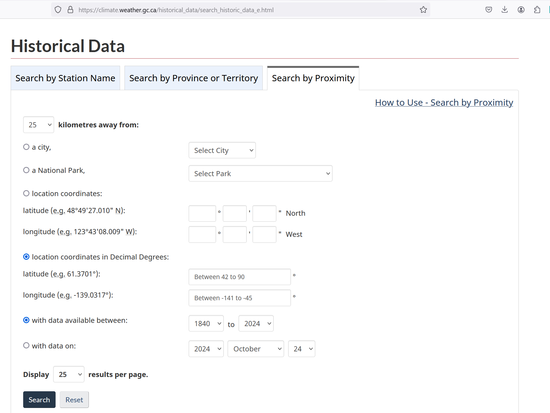
Figure 5.2B. “Search by Proximity” tab on ECCC Historical Data website.
We advise selecting a station no more than 25 km away, but that is also up to the user’s judgement and their responsibility to justify.
It also helps to select a proper range of dates using either “with data available between” or “with data on” option.
From the list of stations pick one that’s has “Hourly” data for the dates you need, and is closest to your location (see example in figure 5.2C):

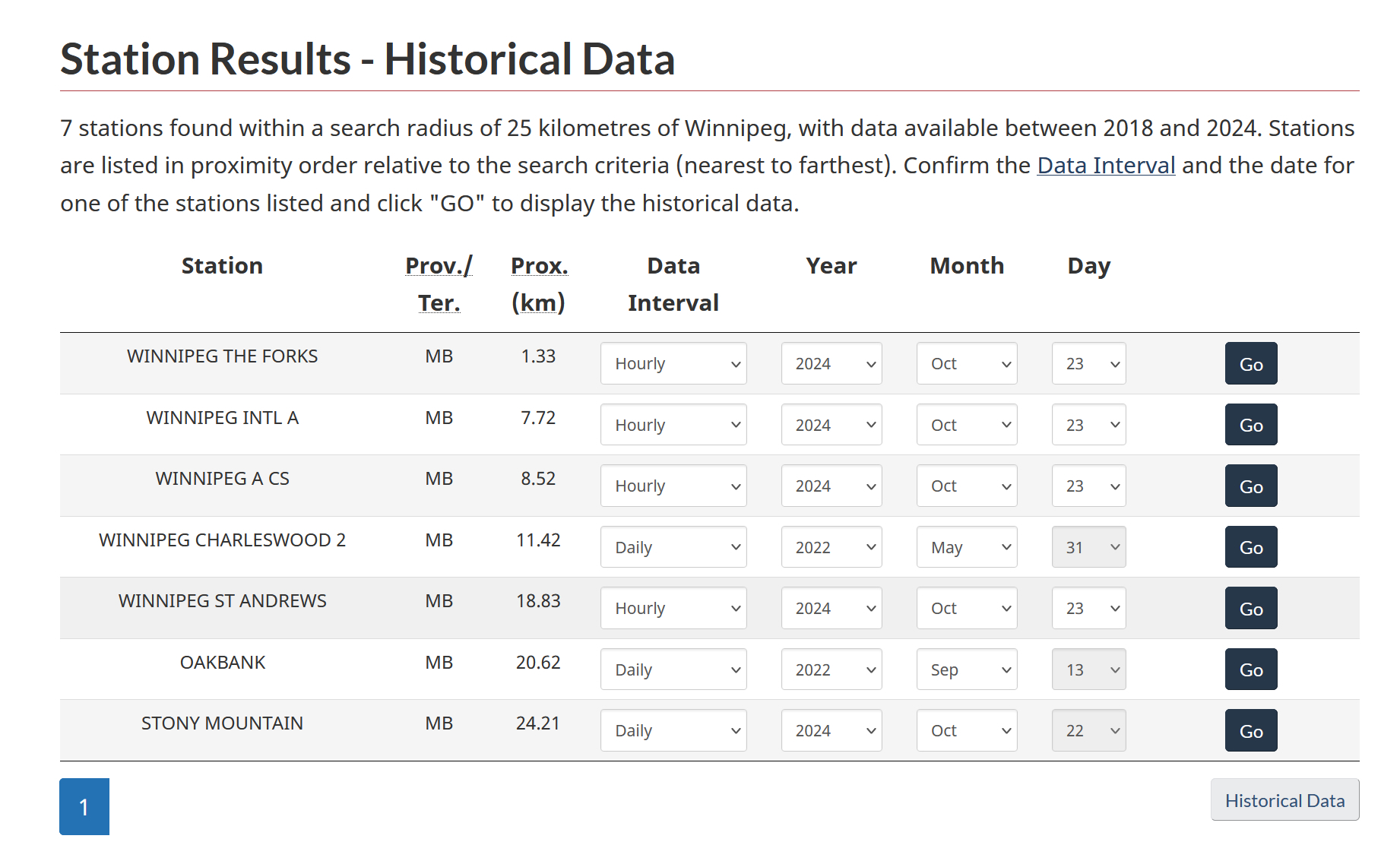
Figure 5.2C. Search results for selecting the station for gap-filling.
In this example, the closes would be “WINNIPEG THE FORKS”; click on “Go”, and make a note of the “Climate ID” number provided (figure 5.2D; in this case, the climate ID is 5023262).

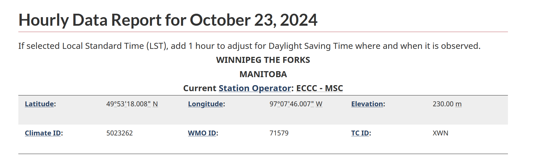
Figure 5.2D. Example of Hourly Data Report for Winnipeg The Forks, showing the Climate ID number.
Next, you need the Station ID (which is different to the Climate ID). Go to this website: https://collaboration.cmc.ec.gc.ca/cmc/climate/Get_More_Data_Plus_de_donnees/; open the Station Inventory EN.csv file and search on the Climate ID number that you saved. The number in the column to the right of this is the Station ID, which in the Winnipeg example is 28051. This Station ID will be used for the data downloads.

Create a script using the snippet below (download code snippet here or copy from below; we recommend adding this into your “main” do-it-all script introduced in section 4.2), and enter your Station ID and other relevant information (years and months). You can enter multiple station IDs at once.

%% get Canadian ECCC station data
 structProject = set_TAB_project(projectPath); 
 stationIDs = [28051]; 
 yearsIn = 2022:2023; 
 monthsIn  = 1:12; 
 for cntStations = 1:length(stationIDs) 
     sID = stationIDs(cntStations); 
     pathECCC = fullfile('yyyy','ECCC',num2str(sID)); 
     try 
         run_ECCC_climate_station_update(yearsIn,monthsIn,sID,structProject.databasePath)     
     catch 
         fprintf('Error processing station: %d (year: %d, month: %d)\n',sID,yearsIn,monthsIn(end)); 
     end 
 end

Running this script will create the database for the given station ID, for two years (2022 and 2023) in the current project folder. The new database for the station 28051 is located here: <projectPath>/Database/2022/ECCC/28051/30min/ (and similarly for 2023).
Alternatively, if a user wants to create the ECCC database just for the current year, or to keep the climate data base up to date by downloading all the months between Jan and the current month, they can use this function call: run_ECCC_climate_station_update([],1:month(datetime),28051,db_pth_root).

Or, for example, to update only the last two months of the current year: run_ECCC_climate_station_update([],month(datetime)-1:month(datetime),28051,db_pth_root).

Create Database Using Data from U.S. Meteorological Stations

For gap-filling met data for U.S. flux sites, you can use data from the U.S. National Centers for Environmental Information (NCEI) climate stations if they are in close proximity.

Some resources to find the nearest NCEI station and its ID:

Map view of stations: https://www.ncei.noaa.gov/access/search/data-search/global-hourly.
Station list can be found at: https://www.ncei.noaa.gov/pub/data/noaa/isd-history.txt.
StationID is the USAF and WBAN numbers combined into an 11-digit number.

Below is some sample code (download code snippet here or copy from below) where you should edit the stationsIDs (can be just one or more), UTC_offset, and yearRng parameters. Again, if you are using this code, we recommend adding it into your “main” do-it-all script introduced in section 4.2.

%% get US station data
% 31km away: 72493023230 (Oakland international airport, 2021-2024, TA&P)
% - Station list can be found at: https://www.ncei.noaa.gov/pub/data/noaa/isd-history.txt
% - stationID is the USAF and WBAN numbers combined into an 11-digit number
% - Map view of ISD stations: https://www.ncei.noaa.gov/access/search/data-search/global-hourly
structProject = set_TAB_project(projectPath); 
stationIDs = {'72493023230'};
UTC_offset = [-8];
yearRng = 2019:2024; 

for cntStations = 1:length(stationIDs) 
    sID = stationIDs{cntStations};
    UTC2local = UTC_offset(cntStations);
    dbPath = fullfile(structProject.databasePath,'yyyy','NCEI',sID); 
    for yearIn = yearRng
        try 
            db_NCEI_climate_station(yearIn,UTC2local,sID,dbPath,'60MIN') 
        catch 
            fprintf('Error processing station: %s, Year: %d\n',sID,yearIn); 
        end 
    end
end

Visualize and inspect your newly created database

Once your database is created, we strongly advise you to review its contents using Biomet.net functions. Some of these are listed in the tutorial under section 4.2, and section 6 provides extensive details of visualization tools for inspecting and analyzing raw and cleaned data.

When you have confirmed that all the traces you expect to see are present in your newly created Database, you are ready to start cleaning the data. First, you need to obtain the set of sample, configuration, and standardization files, described in section.