6.3. Quick Start: Third Stage Cleaning and Converting to Ameriflux Output
Third Stage Cleaning
The third stage cleaning generally requires the least amount of work by the user, but is usually the most computationally intensive stage, as it includes running models for gap-filling fluxes and flux partitioning. The following example assumes you have already completed first and second stage cleaning for one site.
Open your site-specific
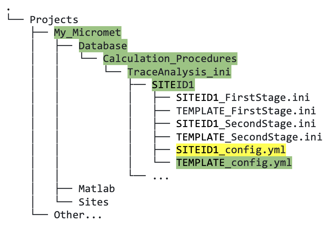
SITEID1_config.ymlfor editing (figure 6.5):
Figure 6.5. Directory tree showing location of third stage custom YAML file that must be copied (green highlighted text) and edited (yellow highlighted text).
At the top of your site-specific configuration file (i.e.,
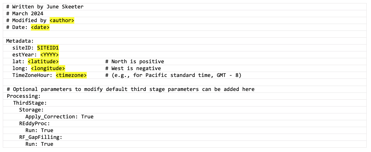
SITEID1_config.yml), input the site ID, the year that measurements at the site began, and the metadata for your site (figure 6.6; yellow highlighted text). ThenorthOffsetcan be found in your site GHG biomet file and this information is used for filtering data by wind direction, to comply with eddy-covariance measurement standards.The peach highlighted text in figure 6.6 indicates parts of the file that should be checked in relation to your site data:
- First, check that the flux variables listed are actually measured at your site, otherwise replace the right hand side with
NULL. - Second, check the met variable names for used for gap-filling are named the same as those output by your second stage cleaning.
- Third, if you wish to, you can edit the wind sector and precipitation filter values, but we recommend the values already written in the file.

Figure 6.6. Third stage site-specific custom YAML file showing which fields to edit in yellow highlighted text, and optional text to check or edit in peach highlighting.
The main configuration file (
global_config.yml) for running third stage cleaning is located in theTraceAnalysis_inidirectory, and generally speaking this should not be edited. The customSITEID1_config.ymlfile can be used to add parameters/inputs; these site-specific settings will overwrite those in theglobal_config.ymlif they are also defined there.- First, check that the flux variables listed are actually measured at your site, otherwise replace the right hand side with
Next, test the third stage data cleaning in Matlab; remember that it can take a lot longer to run than first and second stages. Note that the cleaning stage argument for third stage cleaning is
7(not 3; this is a legacy artifact), as follows:fr_automated_cleaning(yearIn,siteID,7) % third stage
The output will appear in two directories:
ThirdStageandThirdStage_Default_Ustarwithin theCleandirectory, where the second stage output is; again, we recommend that you inspect this data using the visualization tools.
Third stage output: flux variable definitions
The standalone flux variable names (i.e., FCH4, FC, H, LE) are copied directly from the second stage output, then wind sector and precipitation filters are applied to comply with eddy-covariance measurement theory, with no change to the variable name. For the variable names with suffixes following the flux variables, these suffixes represent different algorithms that we have applied sequentially, in the order that they appear. For now, this description provides only definitions, and more detailed information on each output variable will be provided on this webpage soon.
| Suffix | Definition |
|---|---|
| No suffix | Standard cleaning (wind direction and precipitation filtering) |
| _PI_SC | Storage flux Correction |
| _PI_SC_JSZ | Plus z-score filter |
| _PI_SC_JSZ_MAD | Plus Median of Absolute Deviation (about the median) filter |
| _PI_SC_JSZ_MAD_RP | Plus REddyProc applied (u-star filtering) |
This link provides descriptions of suffixes applied to REddyProc output, e.g., _uStar, U95, _orig, and _f.
Output your data to an Ameriflux CSV file
Finally, once you have inspected your clean data and are happy with your INI files, you can output the data to a CSV file formatted for submission to Ameriflux:fr_automated_cleaning(yearIn,SITEID,8) % Ameriflux CSV output
The output will appear in an Ameriflux directory within the Clean directory, where the second and third stage output is.
fr_automated_cleaning(yearIn,SITEID,[1 2 7 8]) % all three stages plus Ameriflux output